2.2 Downloading and Importing HMDA Data in CSV Format
To practice importing CSV files in R, we will use the Home Mortgage Disclosure Act (HMDA) data in CSV format. This data can be found at the Consumer Financial Protection Bureau (CFPB) website. In particular we will be working with the Snapshot National Loan Level Dataset, specifically for that in 2022 for Nevada.
2.2.1 Snapshot National Loan Level Dataset
The Snapshot files contain the national HMDA datasets as of May 1, 2023 for all HMDA reporters, as modified by the Bureau to protect applicant and borrower privacy. The snapshot files are available to download in both .csv and pipe delimited text file formats at the following link: https://ffiec.cfpb.gov/data-publication/snapshot-national-loan-level-dataset/. One of the issues with these files however is that they are quite large, so we will be working with a subset of the data for Nevada in 2022.
The subset of the data for Nevada in 2022 can be downloaded from the following link: Nevada 2022 HMDA Data.
2.3 Importing CSV Files in R
R provides several functions for importing CSV files. The most commonly used function is read.csv(), which is part of the base R package. Additionally, the readr package offers the read_csv() function, which is optimized for faster performance and easier handling of large datasets.
2.3.1 Using read.csv()
The read.csv() function is straightforward to use. It is actually a special case of the more general read.table() function, with default parameters set for reading CSV files Here’s how you can import a CSV file using this function:
# Importing a CSV file using read.csv()
data <- read.csv("downloads/state_NV.csv")

# Display the first few rows of the data
head(data)
In this example, replace "downloads/state_NV.csv" with the actual path to your CSV file. The head() function is used to display the first few rows of the imported data.
Details on read.csv()
The read.csv() function is a simplified wrapper around read.table(), with pre-set arguments tailored for reading comma-separated files. Specifically, it sets the following default arguments:
sep = ","sets the field separator to a comma.header = TRUEindicates that the first line of the file contains column names.stringsAsFactors = default.stringsAsFactors()specifies whether character vectors should be converted to factors (default behavior depends on the R version).
Here’s an equivalent way to use read.table() to achieve the same result as read.csv():
# Importing a CSV file using read.table()
data <- read.table("downloads/state_NV.csv", sep = ",", header = TRUE, stringsAsFactors = FALSE)

# Display the first few rows of the data
head(data)
As you can see, read.csv() simplifies the process by encapsulating these common settings, making it easier and quicker to read CSV files.
2.3.2 Using read_csv() from the readr Package
The readr package provides a faster and more convenient way to import CSV files with the read_csv() function. First, you need to install and load the readr package:
Once the package is installed, you can use the read_csv() function to import the CSV file:
# Load the readr package
library(readr)

# Importing a CSV file using read_csv()
data <- read_csv("downloads/state_NV.csv")

# Display the first few rows of the data
head(data,50)
Similar to read.csv(), replace "downloads/state_NV.csv" with the actual path to your CSV file. The read_csv() function also automatically parses the data types of the columns, which can save you time and effort, you need to be carefull as sometimes read_csv() may guess the column type wrong!
Details on read_csv()
The read_csv() function is a special case of the more general read_delim() function from the readr package, with default parameters set for reading comma-separated files. Specifically, it sets the following default arguments:
delim = ","sets the field separator to a comma.col_types = cols()automatically detects the data types of columns unless specified otherwise.trim_ws = TRUEindicates that whitespace should be trimmed from the beginning and end of each field.
These defaults make read_csv() particularly convenient for reading CSV files without needing to manually specify these common options.
Here’s an equivalent way to use read_delim() to achieve the same result as read_csv():
# Importing a CSV file using read_delim()
data <- read_delim(
  "downloads/state_NV.csv",
  delim = ",",
  col_types = cols(),
  trim_ws = TRUE
)

# Display the first few rows of the data
head(data, 50)
As you can see, read_csv() simplifies the process by encapsulating these common settings, making it easier and quicker to read CSV files.
2.3.2.1 Handling Parsing Issues
If you been following along, when you ran data <- read_csv("downloads/state_NV.csv") you have probably encountered a warning similar to:
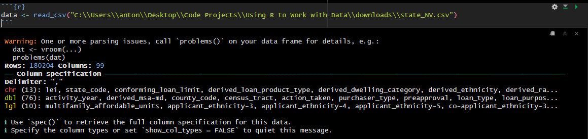
The warning is letting us know that read_csv() ran into some parsing issues, and its recommending that we run problems() to see what the issues are. Let’s run problems() to see what the issues are:
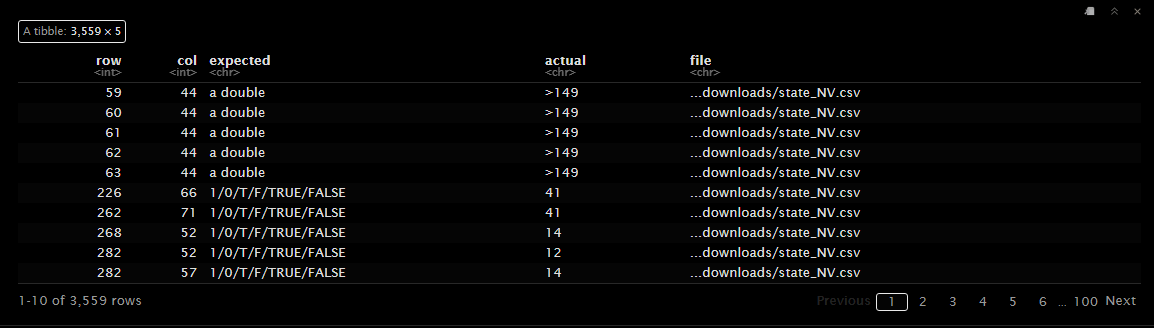
The problems() function displays the issues encountered during parsing. The ‘row’ column indicates the row number where the issue occurred, and the ‘col’ column indicates the column number. The ‘expected’ column shows the expected data type, and the ‘actual’ column shows the actual value.
In the example above in row 59, column 44 expected a double but the cell contains “>149”, which is a character type. A double is a numeric data type that can represent decimal numbers, while a character is a text data type. The issue here is that read_csv() expected a double but found a character. Even though you can’t see it in the table above Column 44 is the total_units column, which should contain the total number of units for the property. The value “>149” lets us know that the property has more than 149 units. Therefore the correct column type should be character and not double.
There are two main ways to handle parsing issues in read_csv():
- Manually Specify Column Types: You can manually specify the column types using the
col_typesargument inread_csv(). This approach is useful when you know the data types of the columns in advance, but might be cumbersome for large datasets with many columns. - Increase the
guess_maxArgument: You can increase theguess_maxargument inread_csv()to allow the function to guess the column types for a larger number of rows. This approach isn’t perfect, but this way you can avoid having to manually specify the column types.
Below is a code example to manually specify the column types:
# Manually specify the column types
data <- read_csv(
  "downloads/state_NV.csv",
  col_types = cols(
    loan_amount = col_double(),
    total_units = col_character(),
    .default = col_character(),
  ),
  na = c("", "NA") # This is to specify what is considered a missing value
  )
In this code, we manually specify the column types for the loan_amount and total_units columns. We also set the default column type to col_character() to ensure that all other columns are treated as character columns. The na argument specifies the values that should be treated as missing values, which in this case we have set to an empty string and “NA”.
It’s also possible to set the guess_max argument to a higher value to allow read_csv() to guess the column types for a larger number of rows. This can be useful when you have a large dataset and want to avoid manually specifying the column types. You can even set it to Inf to allow read_csv() to guess the column types by using all the rows in the dataset.
2.3.3 Handling File Paths
When specifying the path to your CSV file, it’s important to ensure that the path is correct. You can use absolute paths or relative paths. Here are some examples:
- Absolute Path: An absolute path specifies the complete path from the root directory. For example, on Windows:
"C:/Users/YourName/Documents/data.csv", or on macOS/Linux:"/Users/YourName/Documents/data.csv". - Relative Path: A relative path specifies the path relative to your current working directory. For example, if your current working directory is
"C:/Users/YourName/Documents", you can use"data.csv".
You can check your current working directory in R using the getwd() function:
You can also set the working directory using the setwd() function:
2.3.4 Common Issues and Solutions
- File Not Found Error: Ensure the file path is correct and the file exists at the specified location.
- Incorrect Data Parsing: If columns are not parsed correctly, you can specify the column types manually using the
col_typesargument inread_csv(). - Missing Values: R automatically handles missing values as
NA. You can customize the handling of missing values using thenaargument.
By understanding how to import CSV files in R, you can easily load your data and start your data analysis process. In the next sections, we will explore how to clean and manipulate the imported data to prepare it for analysis.