Chapter 5 Basic Regression Analysis in R
5.1 Introduction
Regression analysis is a powerful statistical method used to examine the relationship between a dependent variable and one or more independent variables. In this chapter, we will explore how to perform basic regression analysis in R using the HMDA (Home Mortgage Disclosure Act) dataset. Specifically, we will use the income variable to predict property_value.
5.1.1 Preparing the Data
Before performing regression analysis, it’s crucial to ensure that the data is clean and properly formatted. We’ll start by loading the necessary packages and preparing the HMDA data.
library(ggplot2)
library(dplyr)
library(readr)

# Load HMDA data
hmda_data <- read_csv("downloads/state_NV.csv", guess_max = Inf)

# Filter and prep HMDA data for regression analysis
filtered_hmda_data <- hmda_data %>%
  filter(
    action_taken == 1,
    loan_purpose == 1,
    occupancy_type == 1,
    lien_status == 1,
    total_units == "1",
    !property_value %in% c("Exempt", NA),
    income <= 250 & income > 0
  ) %>%
  mutate(
    property_value = as.numeric(property_value),
    loan_type = case_when(
      loan_type == 1 ~ "Conventional",
      loan_type == 2 ~ "FHA",
      loan_type == 3 ~ "VA",
      loan_type == 4 ~ "USDA"
    )
  ) %>%
  filter(property_value < 1000000)
5.2 Simple Linear Regression
Simple linear regression is used to model the relationship between two continuous variables. In this case, we will model the relationship between income (independent variable) and property_value (dependent variable).
5.2.1 Fitting the Model
We use the lm() function to fit a linear model.
# Fit the linear regression model
lm_model <- lm(property_value ~ income, data = filtered_hmda_data)

# Display the summary of the model
summary(lm_model)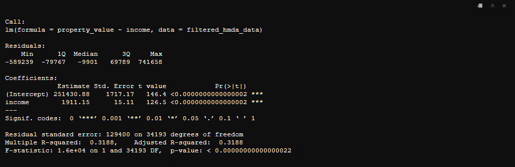
5.2.2 Interpreting the Results
Let’s interpret the results of the simple linear regression model using the provided output.
Coefficients
The Coefficients section provides the estimated values of the intercept and slope in the regression equation:
Intercept: 251,430.88
- This represents the estimated property value when
incomeis zero.
- This represents the estimated property value when
Income: 1,911.15
- This represents the estimated change in property value for each unit increase in
income.
- This represents the estimated change in property value for each unit increase in
Statistical Significance
The Pr(>|t|) column provides the p-values for the coefficients:
Intercept: The p-value is less than 0.0000000000000002, indicating that the intercept is statistically significant.
Income: The p-value is also less than 0.0000000000000002, indicating that
incomeis a statistically significant predictor ofproperty_value.
Model Fit
Residual standard error: 129,400 on 34,193 degrees of freedom
- This represents the average distance that the observed values fall from the regression line.
Multiple R-squared: 0.3188
- This indicates that approximately 31.88% of the variance in
property_valuecan be explained byincome.
- This indicates that approximately 31.88% of the variance in
Adjusted R-squared: 0.3187
- This is similar to the R-squared value but adjusted for the number of predictors in the model.
F-statistic: 1.6e+04 on 1 and 34,193 DF, p-value: < 0.00000000000000022
- This indicates that the model is statistically significant overall.
The results suggest that there is a statistically significant positive relationship between income and property_value. For every unit increase in income, the property_value is expected to increase by approximately 1,911.15 units, holding other factors constant. The R-squared value indicates that income explains about 31.88% of the variability in property_value, which suggests that other factors not included in the model may also play a significant role in determining property values.
Visualizing the Regression Line
We can visualize the regression line using ggplot2.
ggplot(data = filtered_hmda_data, aes(x = income, y = property_value)) +
  geom_point() +
  geom_smooth(method = "lm", color = "red", formula = y ~ x) +
  labs(title = "Regression Line: Property Value vs Income",
       x = "Income (in Thousands of Dollars)",
       y = "Property Value")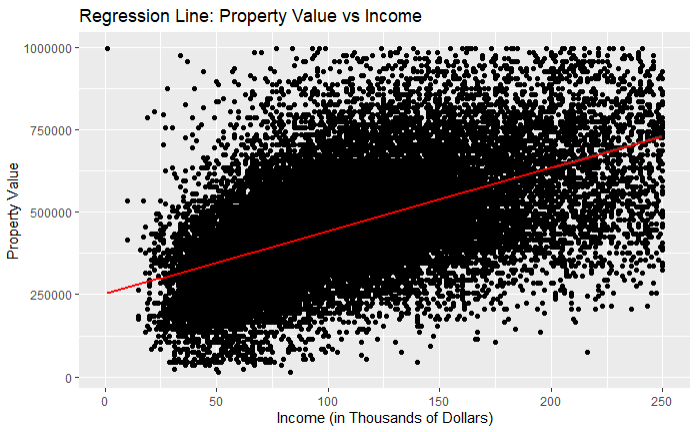
In this plot:
geom_point()adds the data points.geom_smooth(method = "lm", color = "red", formula = y ~ x)adds the regression line with the color red and using the formulay ~ x.
Plotting Residuals Using lm()
You can plot residuals of a linear model fitted with lm() using several methods in R. One common way is to use base R plotting functions to create diagnostic plots. Here is how you can plot the residuals:
- Basic Residual Plot: Plotting residuals versus fitted values.
# Fit the linear regression model
lm_model <- lm(property_value ~ income, data = filtered_hmda_data)

# Plot residuals vs. fitted values
plot(lm_model$fitted.values, lm_model$residuals,
     xlab = "Fitted Values",
     ylab = "Residuals",
     main = "Residuals vs Fitted Values")
abline(h = 0, col = "red")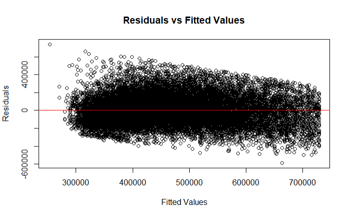
- Diagnostic Plots Plotting multiple diagnostic plots at once.
# Fit the linear regression model
lm_model <- lm(property_value ~ income, data = filtered_hmda_data)

# Produce diagnostic plots
par(mfrow = c(2, 2)) # just lets R know we want the plots to be in 2x2 structure
plot(lm_model)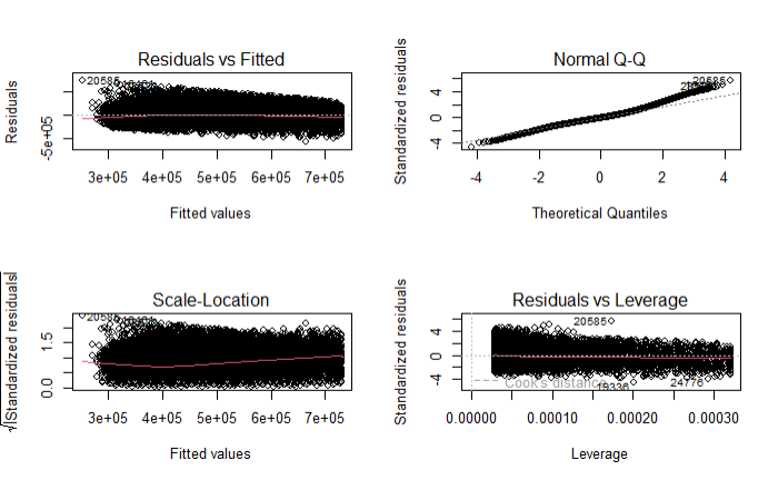
The plot(lm_model) function produces four diagnostic plots:
Residuals vs Fitted
Normal Q-Q
Scale-Location (Spread-Location)
Residuals vs Leverage
These plots help to assess the fit of the model and to identify any potential issues such as non-linearity, heteroscedasticity, and influential observations.
5.3 Multiple Linear Regression
Multiple linear regression is used to model the relationship between a dependent variable and two or more independent variables. In this section, we will extend our analysis to include additional predictors and dummy variables.
5.3.1 Including Multiple Variables
To include more than one independent variable in our model, we simply add them to the formula. For instance, we might want to include both income and loan_amount as predictors of property_value.
5.3.2 Creating Dummy Variables
Dummy variables are used to include categorical variables in the regression model. For example, the loan_type variable in our dataset is categorical, and we need to convert it to dummy variables.
5.3.3 Preparing the Data
We will modify our previous data preparation steps to include additional variables and create dummy variables for loan_type.
# Create dummy variables for loan_type
filtered_hmda_data <- filtered_hmda_data %>%
  mutate(
    loan_type_conventional = ifelse(loan_type == "Conventional", 1, 0),
    loan_type_fha = ifelse(loan_type == "FHA", 1, 0),
    loan_type_va = ifelse(loan_type == "VA", 1, 0),
    loan_type_usda = ifelse(loan_type == "USDA", 1, 0)
  )
5.3.4 Fitting the Multiple Linear Regression Model
We use the lm() function to fit a multiple linear regression model.
# Fit the multiple linear regression model
mlm_model <- lm(property_value ~ income + loan_amount + loan_type_conventional + loan_type_fha + loan_type_va + loan_type_usda, data = filtered_hmda_data)

# Display the summary of the model
summary(mlm_model)
As we can see now instead of just having a coefficients and statistics for the intercept term and income we now also have coefficients for the the dummy variables we created based on the different loan types.
5.4 Robust Linear Regression
Introduction to Robust Regression {.unlisted .unumbered} Robust regression is a technique used when the assumptions underlying ordinary least squares (OLS) regression are violated. These assumptions include the presence of normally distributed errors, constant variance (homoscedasticity), and the absence of outliers. In cases where the data contains outliers or exhibits heteroscedasticity (non-constant variance), OLS estimates can be significantly biased or inefficient.
The rlm() function from the MASS package provides a robust alternative to OLS regression through the use of M-estimators. Unlike OLS, which minimizes the sum of squared residuals, rlm() minimizes a weighted sum of residuals, where weights are adjusted to reduce the influence of outliers. This adjustment allows rlm() to provide more reliable parameter estimates when dealing with problematic data conditions. 3
5.4.1 Preparing the Data
We’ll use the same HMDA dataset prepared for the basic regression analysis.
5.4.2 Fitting the Robust Linear Model
We use the rlm() function from the MASS package to fit a robust linear model.
library(MASS)

# Fit the robust linear regression model
rlm_model <- rlm(property_value ~ income, data = filtered_hmda_data)

# Display the summary of the model
summary(rlm_model)
The interpretation of summary is the same as it was when we ran a simple linear regression using the lm() model. One of the key differences is that you won’t see an R2 statistic. since rlm() down-weight outliers the traditional calculation of R2 would not accurately reflect the model’s fit or explanatory power.
For a more advanced and comprehensive explanation of how
rlm()works you may refer to https://www.researchgate.net/publication/224817420_Modern_Applied_Statistics_With_S↩︎